Welcome to the second part of our credit cart tutorial. You can find the first part
here.
Now it's time to train other models.
We are gonna use:
- Decision tree
- Naive Bayes
- Support vector machine (SVM)
- Random Forest
- Gradient Boosting
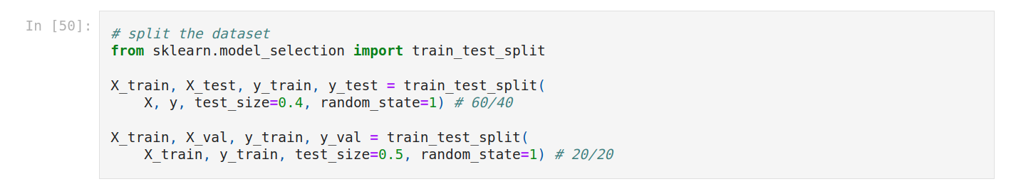
First, we split the dataset into 3 parts (train, validation, and test). So first train, test, then validation, test.
We load the dataset. We create a variable named train with the file path, and create a new variables named df_train to create a dataframe.
Now we fit again logistic regression.
And we instantiate the other algorithms, then train them. And finally, we evaluate them.
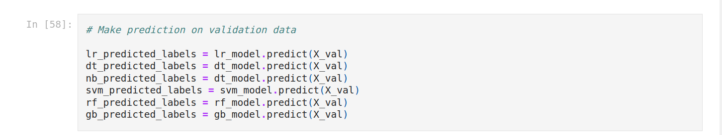
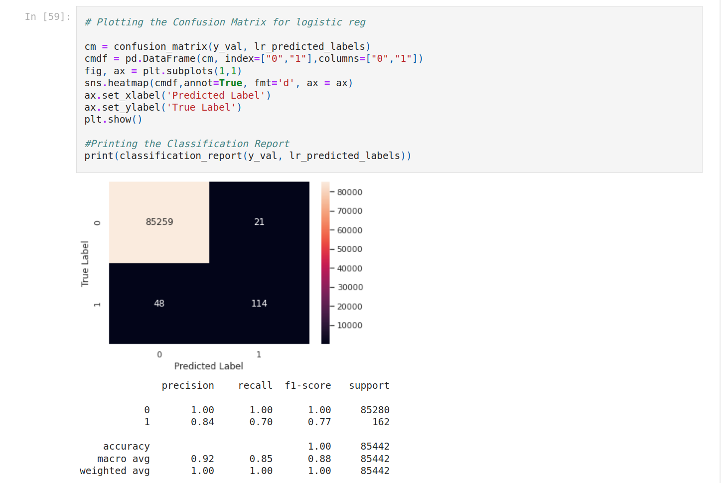
First, we make predictions on validation data for each model.
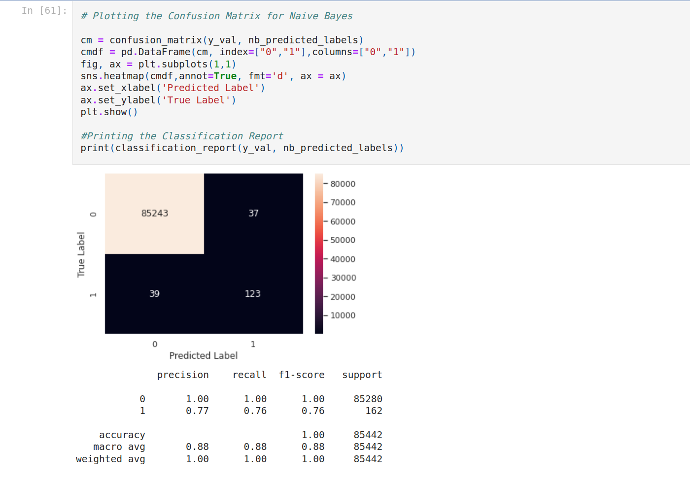
Then plot the confusion matrix for each model.
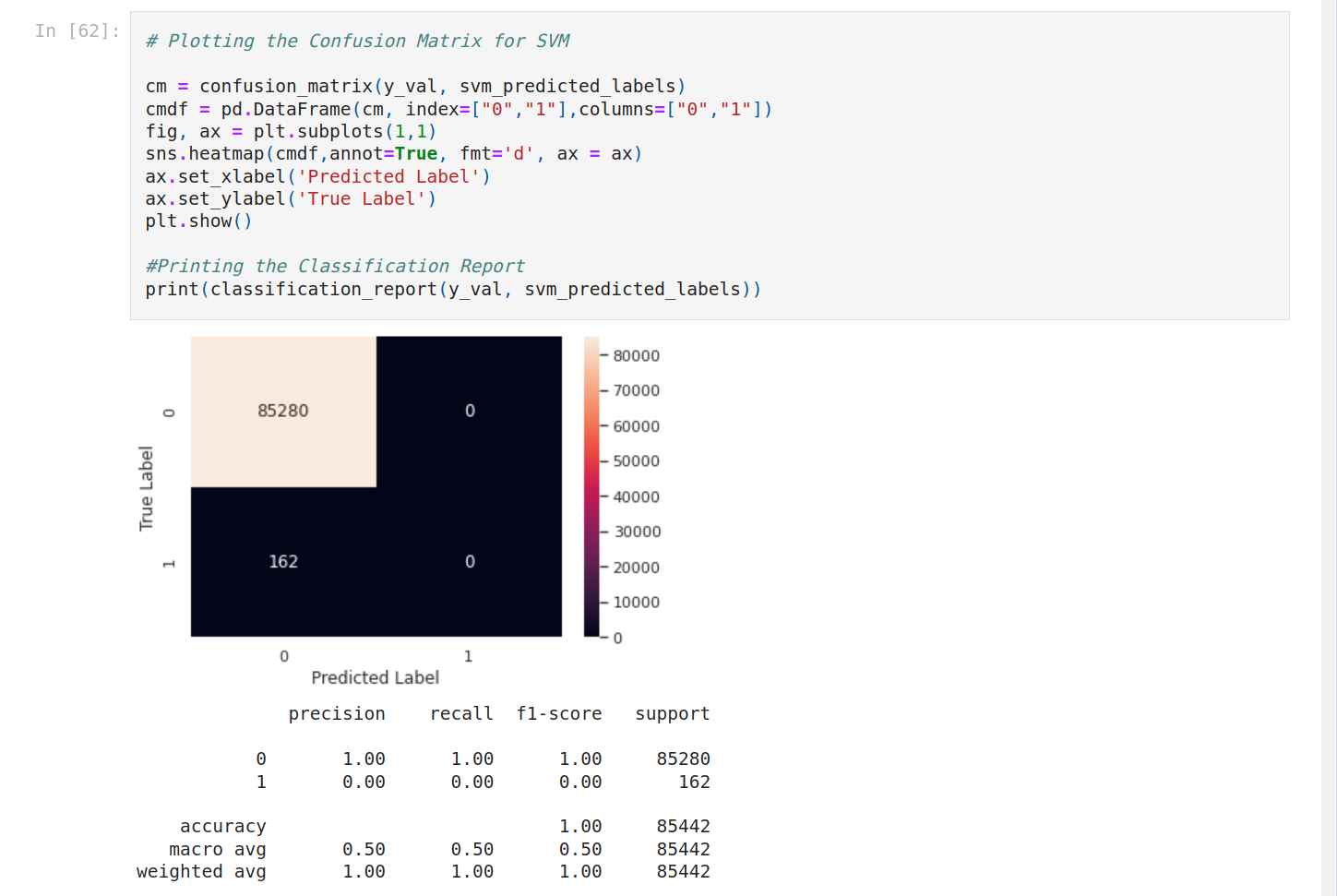
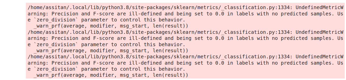
It seems to have a problem with SVM. Let's focus on the other models.

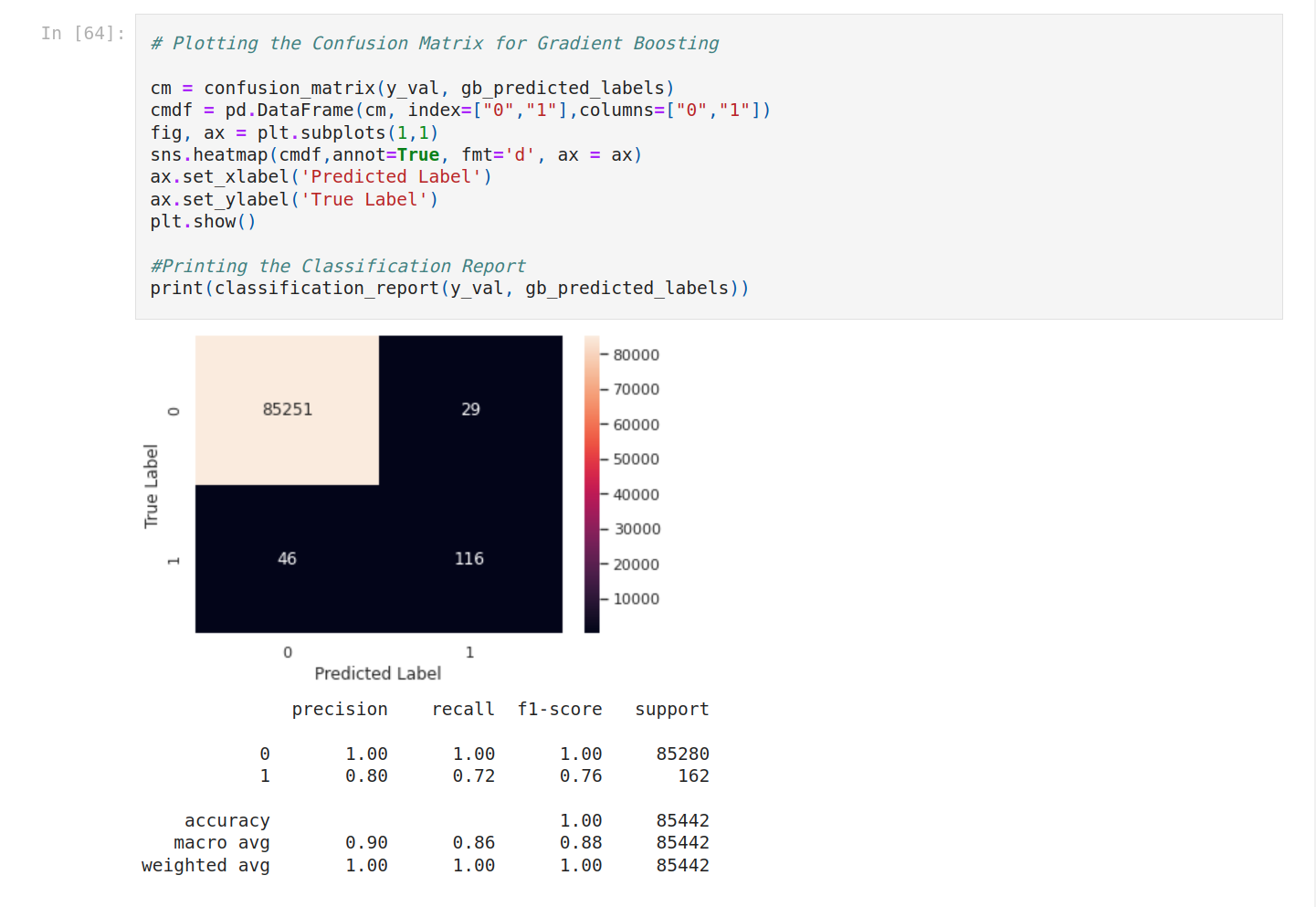
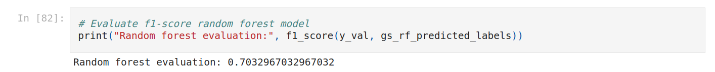
To see better, let’s compare the F1-score.
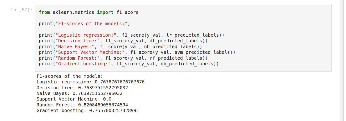
Random forest is the best score!
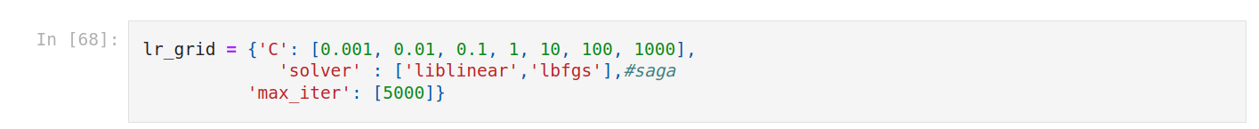
We can do hyperparameter tuning to improve the score. I want to improve the score of logistic regression and random forest. We can use random RandomizedSearchCV (for logistic regression) and GridSearchCV. First we create a grid.
Then set up random hyperparameter search for Logistic regression. Train the new model.
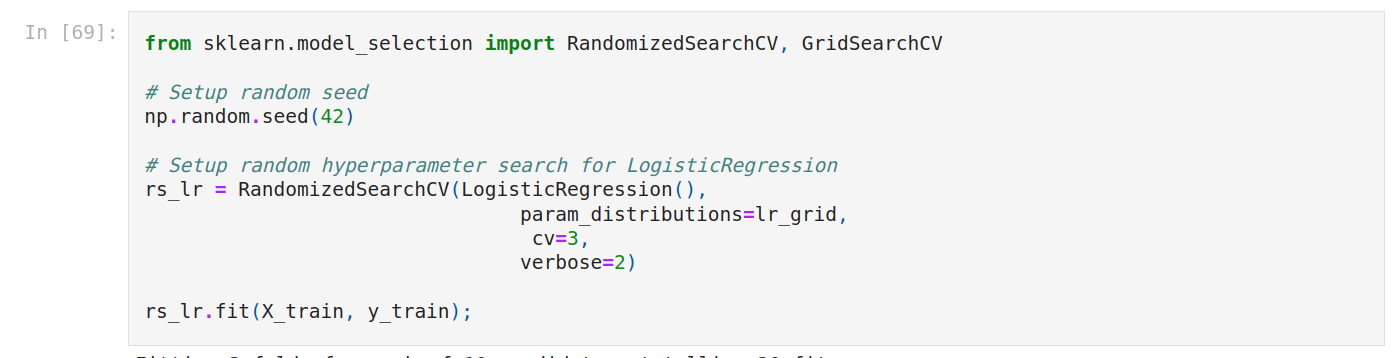
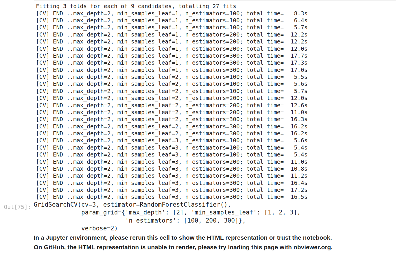
We have to wait a few minutes.
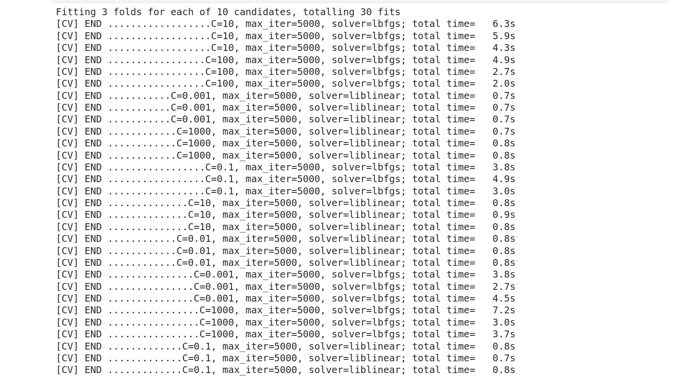
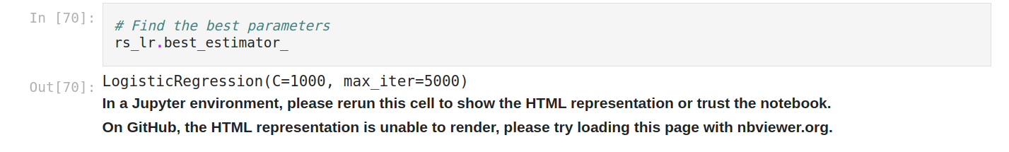
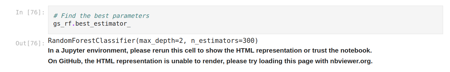
Find the best parameters and predict on evaluation data.
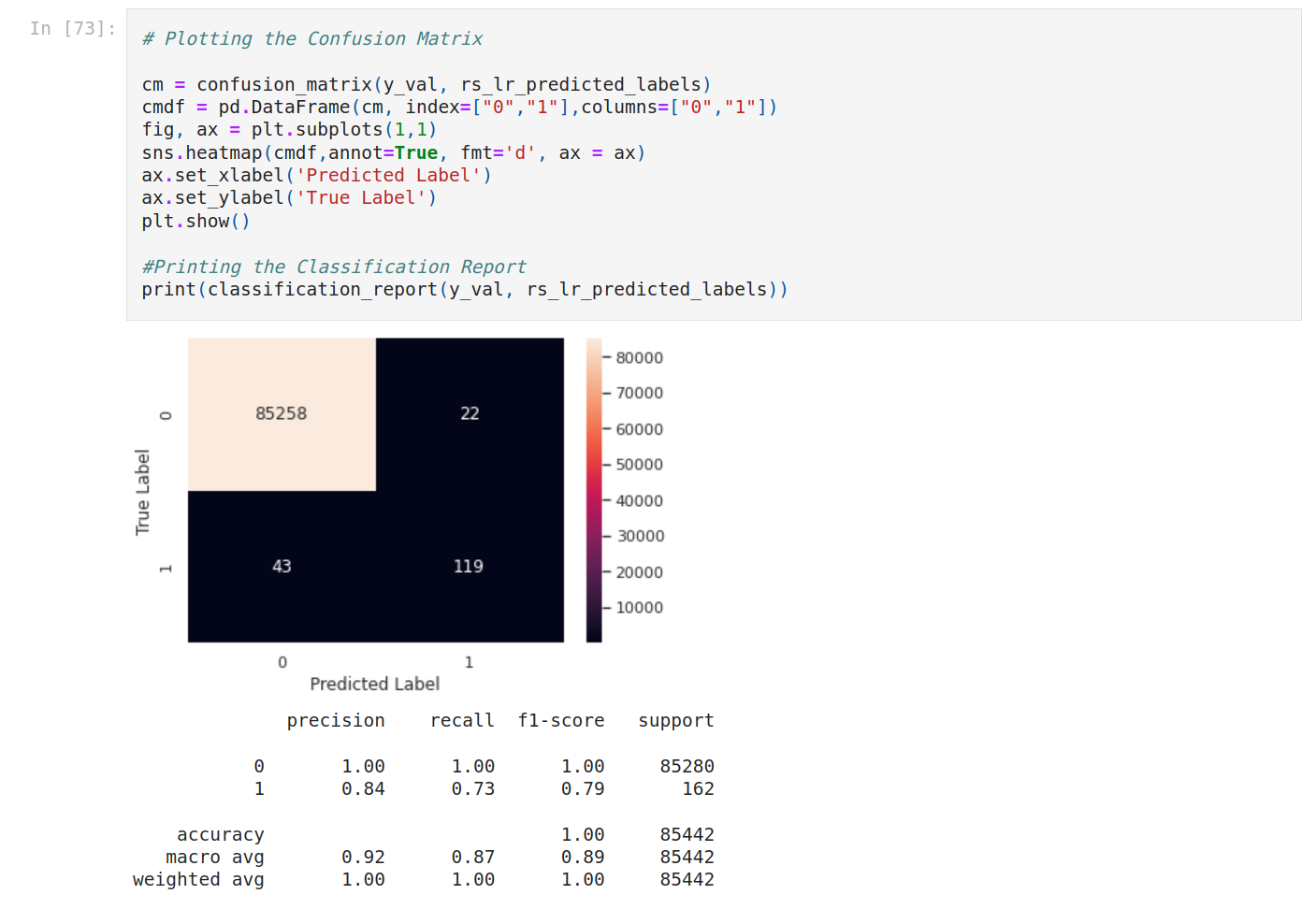
Then plot the result.
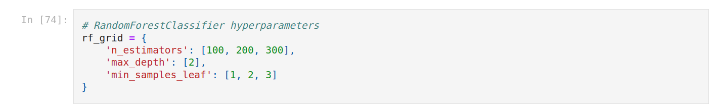
We do the same for random forest with GridSearchCV.

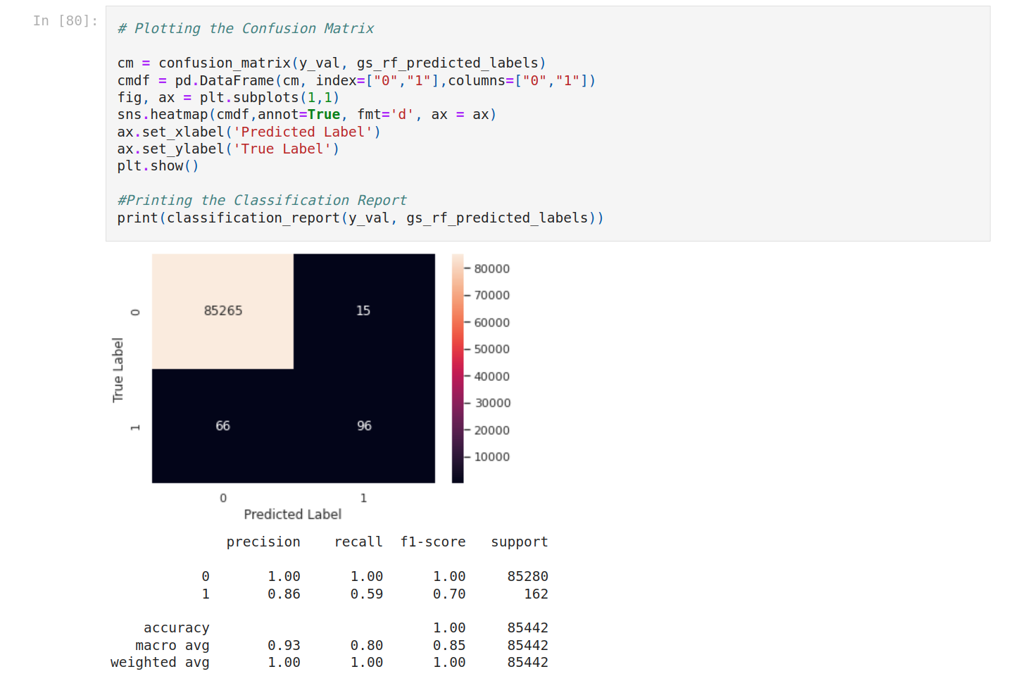
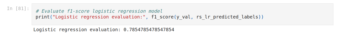
We compare F1 scores.It’s better for logistic regression but worse for random forest. It could be complicated to find the best grid. The problem is that it takes time to process. So we stop here.
Let’s plot ROC curve.
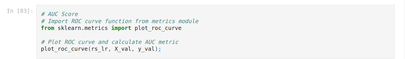
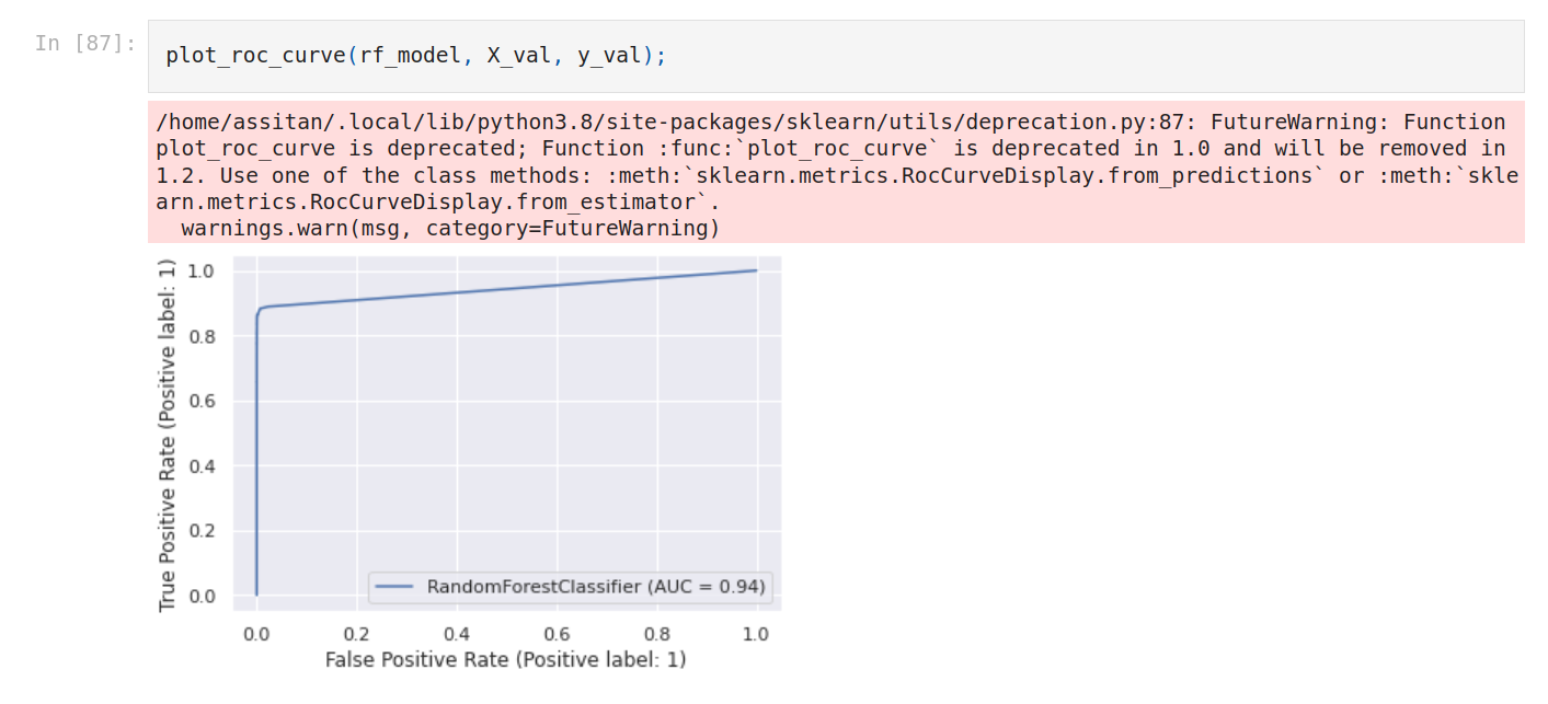
As seen above the area under the ROC curve varies from 0 to 1, with 1 being ideal and 0.5 being random. An AUC (Area Under the ROC Curve) of 0.9 is indicative of a reasonably good model; 0.8 is alright, 0.7 is not very good, and 0.6 indicates quite poor performance. The score is indicative of how good the model separates positive and negative labels.
Logistic regression is better. We’re gonna use the first model with Random forest.
Now let’s test the model. We do the same as evaluation.
We make predictions on test data (probability).
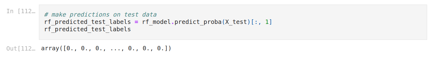
The output is a matrix with predictions. For each credit card, it outputs two numbers, which are the probability of being non fraudulent and the probability of being fraudulent. We select the second column, we don't need both (the probability of being fraudulent).
Let’s use the model. We’re gonna select a credit card from the test data. Let’s display it as a dict so you see the data.
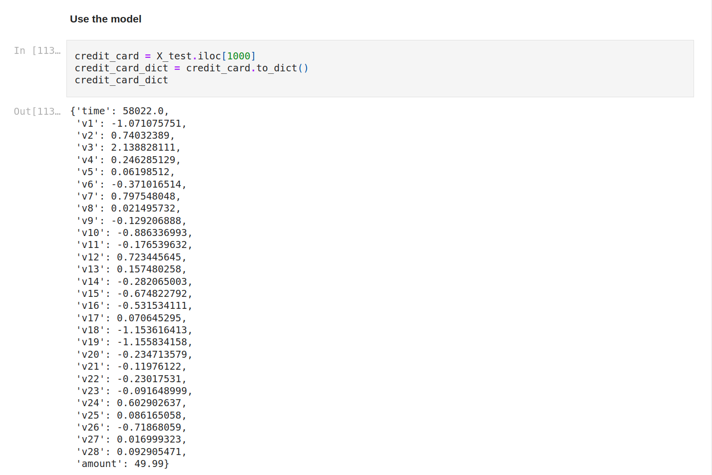
Now we make a prediction on this credit card. This time, there's just one row and we get the second column so we set just zero.
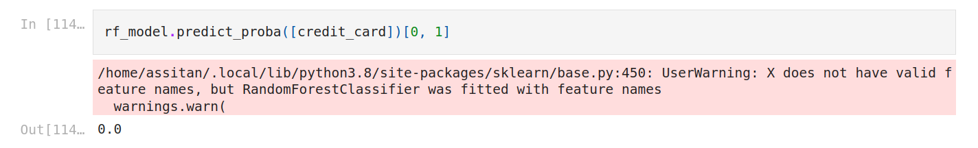
We get zero.
Let’s check the result.
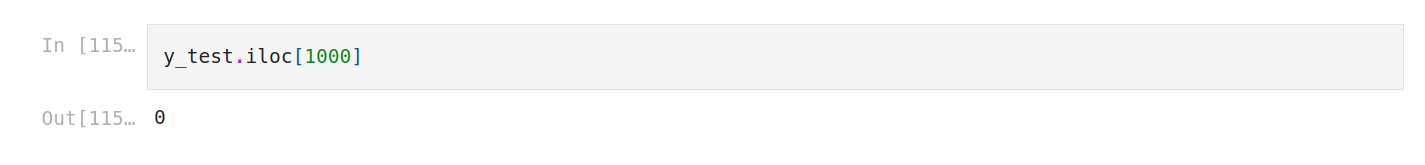
Also zero. So our model had guessed well.
That's it.
What you can do now is deploy the model or improve the score. To improve the score, you can do some feature engineering or try other combinations for the hyperparameters.