How do we know when a credit card is fraudulent or not?
This is a classification problem statement.
I like typing the problem statement, so let’s write in markdown what we’ve said before, whether this credit card is fraudulent or not. Now, about the dataset. We can find it on Kaggle. There is some information about it. Class 0, 1. the statistics. You can download the dataset here to get the archive.
To get it, just click on download, then unzip the archive to get this CSV file.
1. Importing Libraries
We import numpy as np (for algebraic operations on arrays), pandas as pd (for data exploration and manipulation). Then matplotlib, seaborn plotting libraries. The inline is a magic function for visualisation.
2. Loading the dataset
We load the dataset. We create a variable named train with the file path, and create a new variables named df_train to create a dataframe.
3. Exploratory data analysis
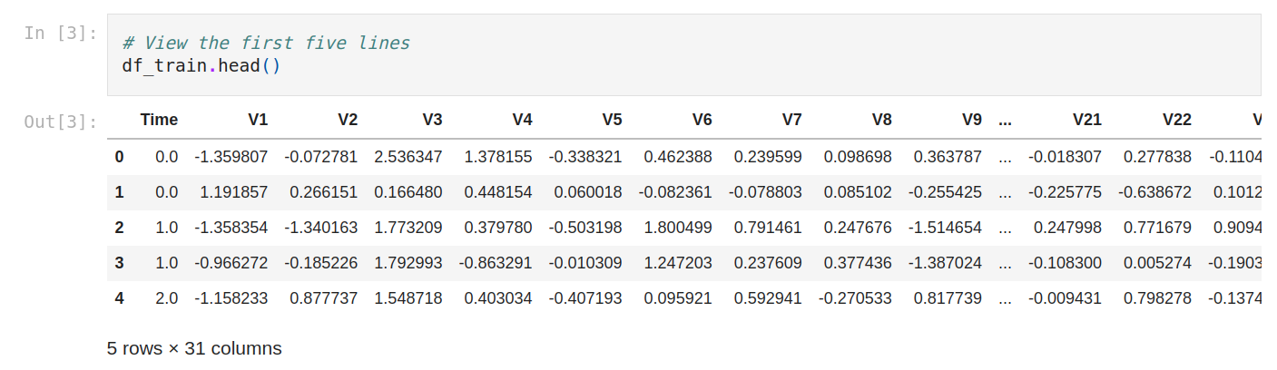
Let’s view the first five lines. For that, we use .head(). at first glance, we see numerical values. We don’t understand the data. so it seems to be changed with PCA. It’s normal because credit card data needs to be confidential.
Now let’s see the shape., A lot of lines.
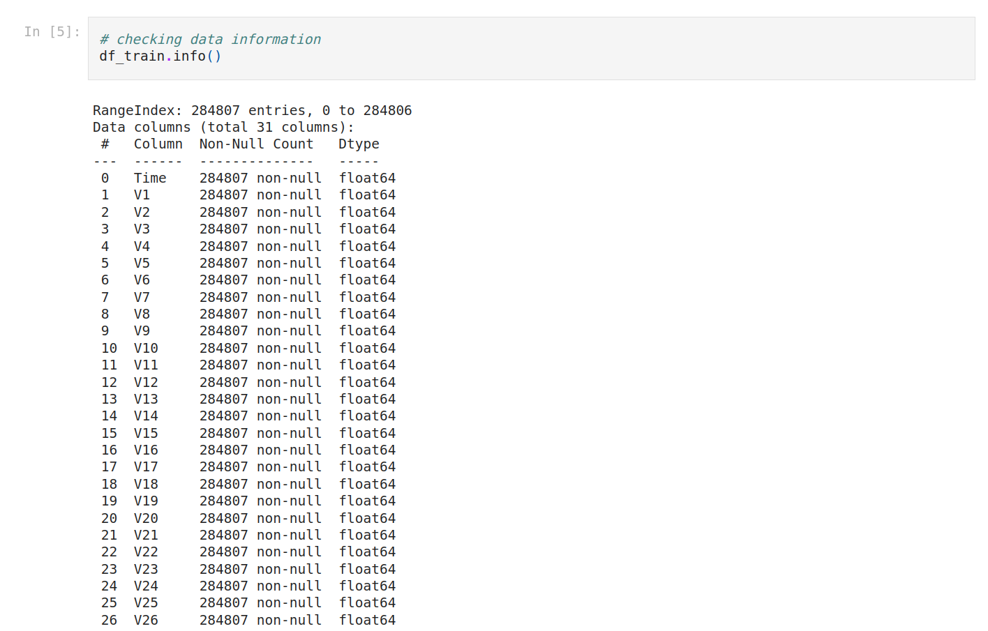
We check the data information. It will help us to to interpret a little bit. So we have 284807 rows, 31 columns, all numerical features and no missing columns.
Let’s type that.
“Interpreting Data Information
We have 284807 rows, any column that contains a lesser number of rows has missing values.
We have 31 columns.
There are numerical features that have data type float64.
There are numerical features that have data type int64.
No missing columns.”
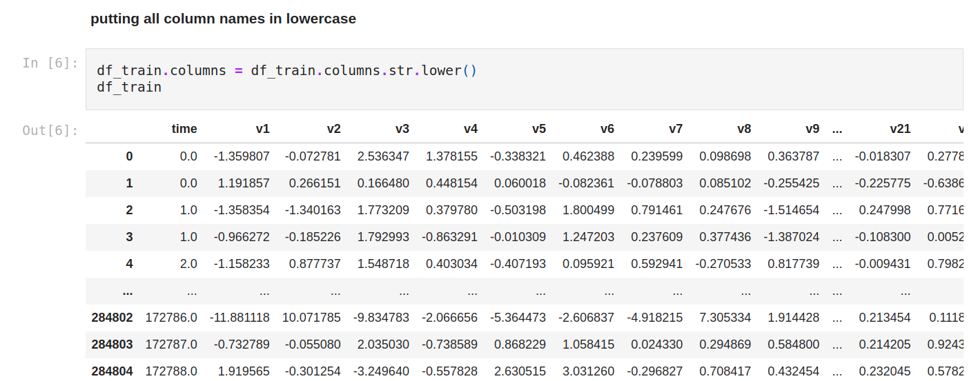
The columns’ names are a little bit different, so let’s normalize everything in lowercase.
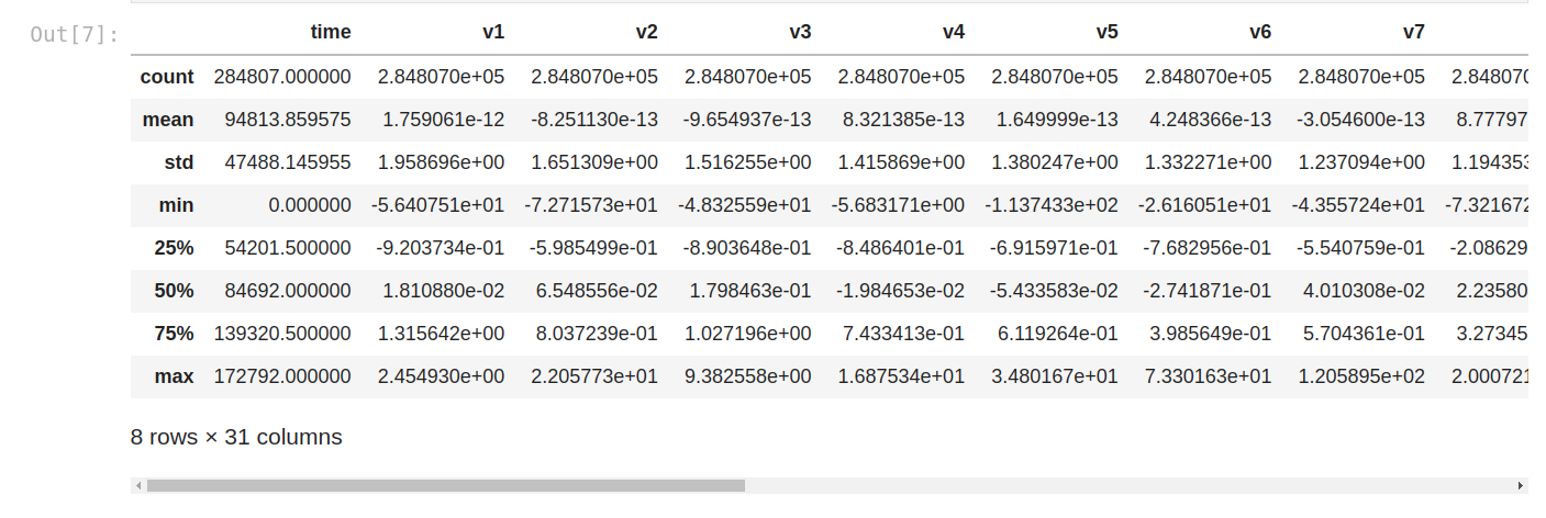
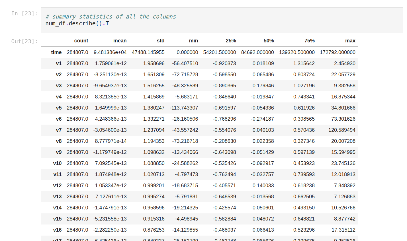
Let’s see the statistics of numerical variables (so every variable).
We can compare the mean of each column with the min/max value, to check if we might have outliers as there's a considerable difference between the average value and the max value.
We can compare the general mean and standard deviation to see if we need to normalize the data as there's a considerable difference between all of them.
Now, we’re gonna go with univariate analysis.
For numerical continue variables, we can use a histogram or scatter plot, for categorical data, we commonly prefer bar plots or pie charts.
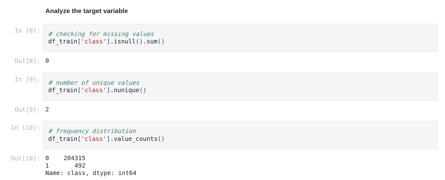
The goal is to analyze the target variable.
We can check again for missing values. Yes, still zéro! We can check the number of unique values and the frequency distribution.
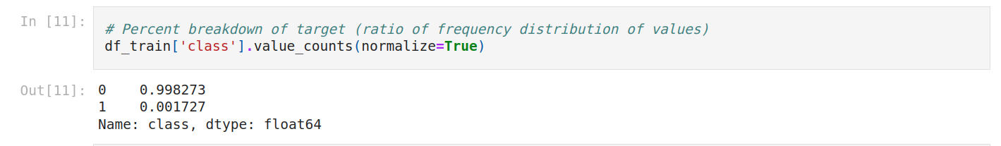
The percent breakdown of the target. As you can see, this is the same code as the frequency distribution, but we normalize it as true.
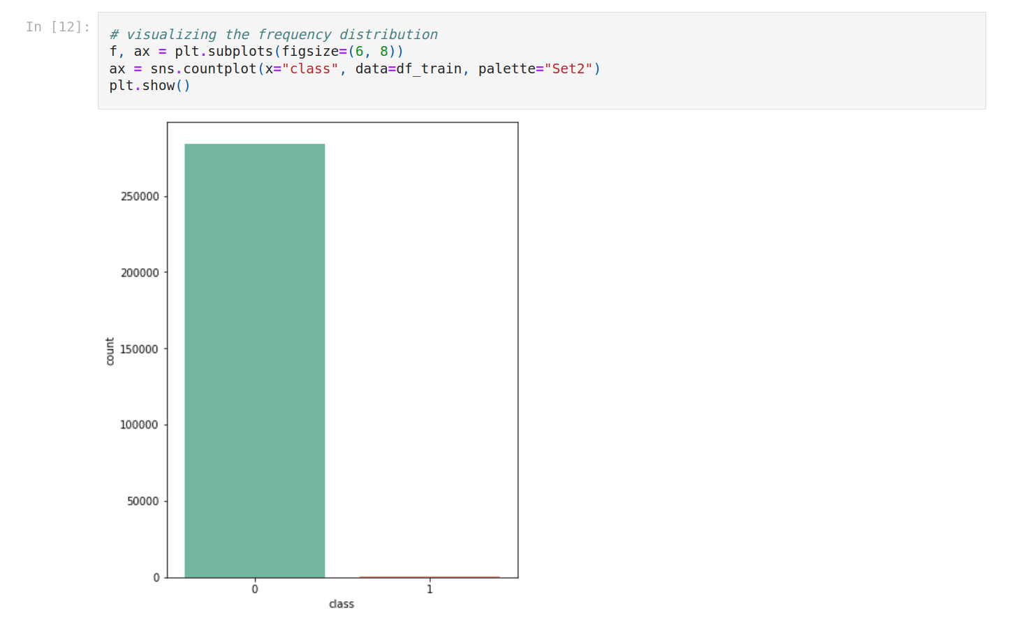
I think it would be better to plot it, so let’s do that.
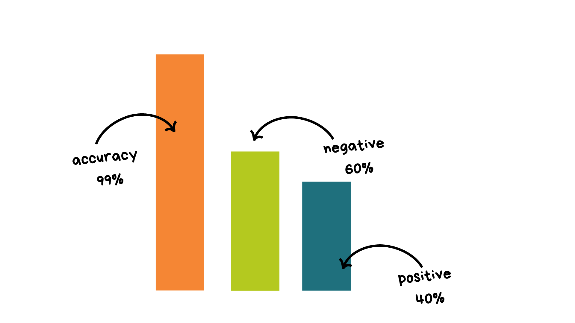
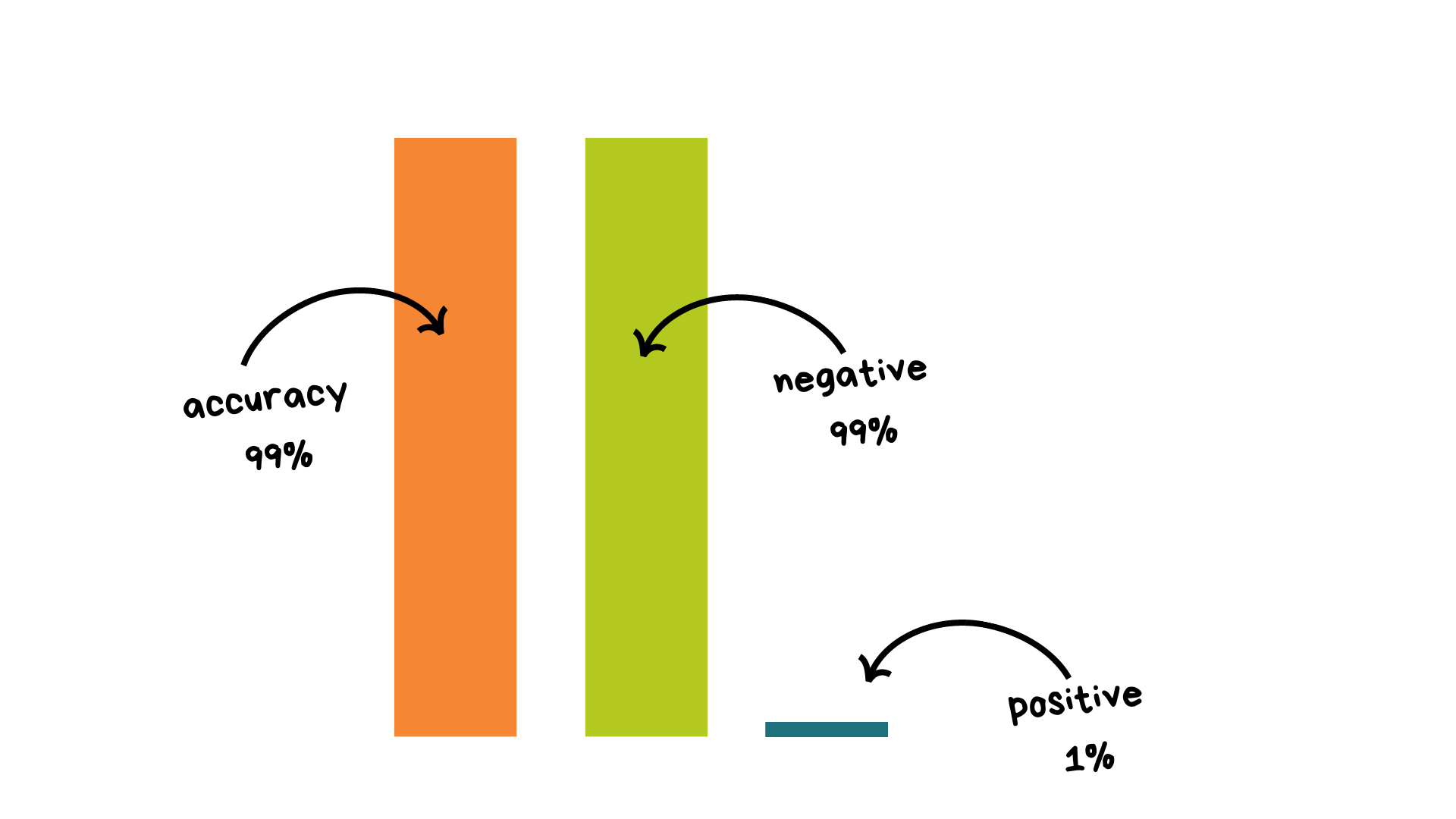
The dataset is very imbalanced (99/1) we can't use accuracy because of the huge imbalance.
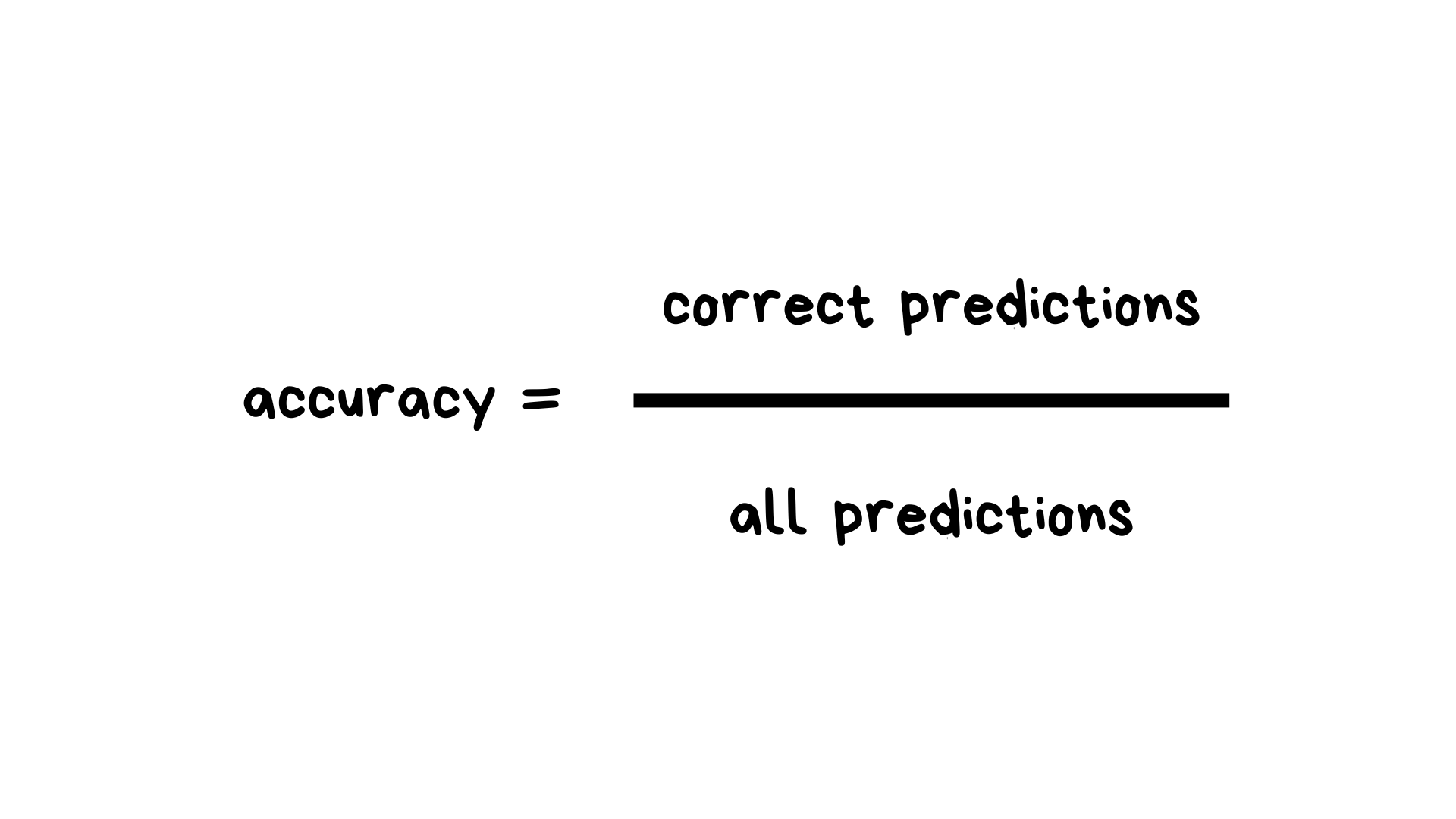
Accuracy is correct predictions on all predictions. Super simple.
This is a balanced dataset.
The thing is, we want to create a baseline model to have a minimum score to beat after with better models. If we have 99% of negative values, our score will be around this number, and how can we beat that? This is too high.
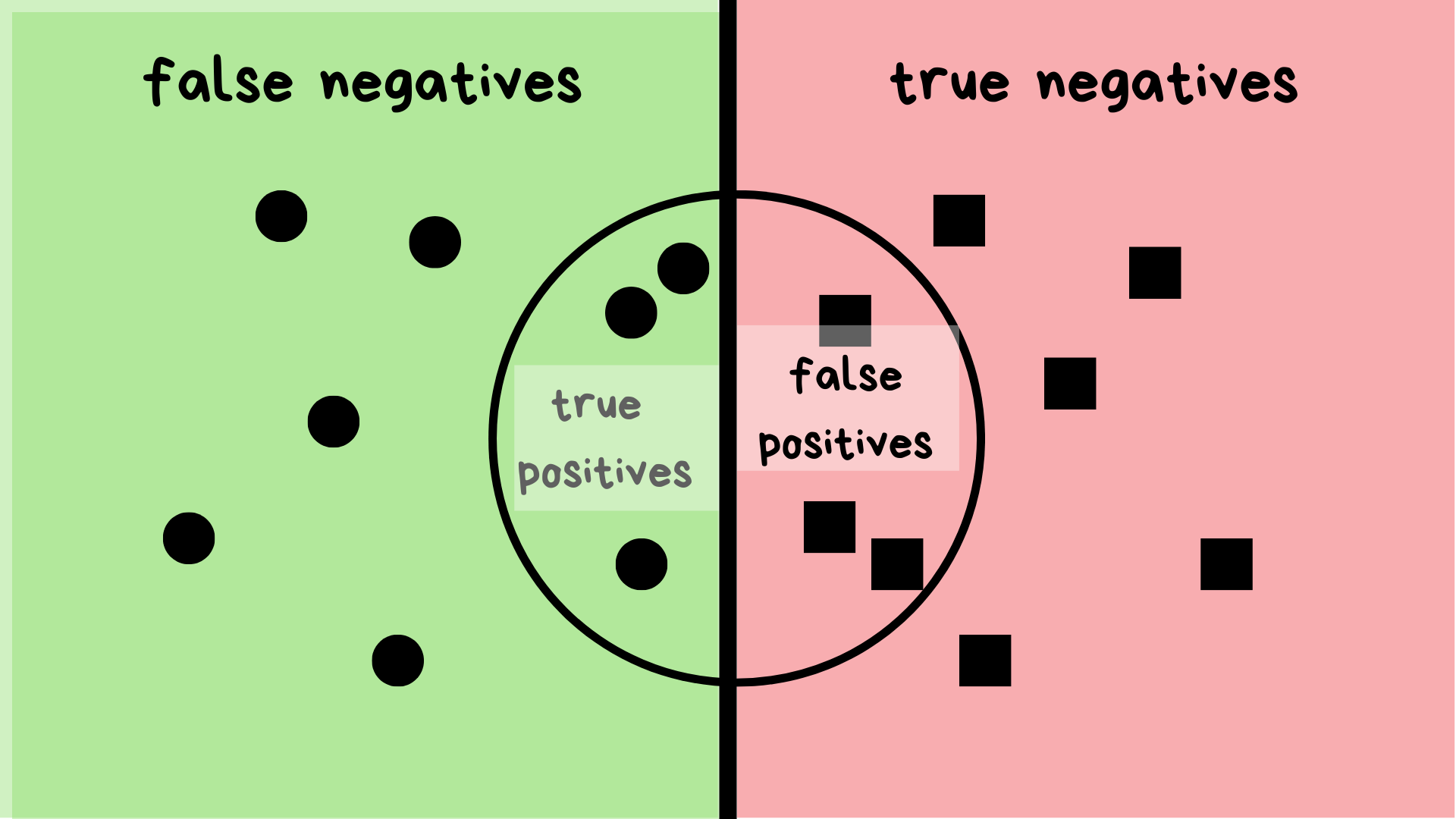
So, we have positive and negative values, and I think you know true positives, false positives….
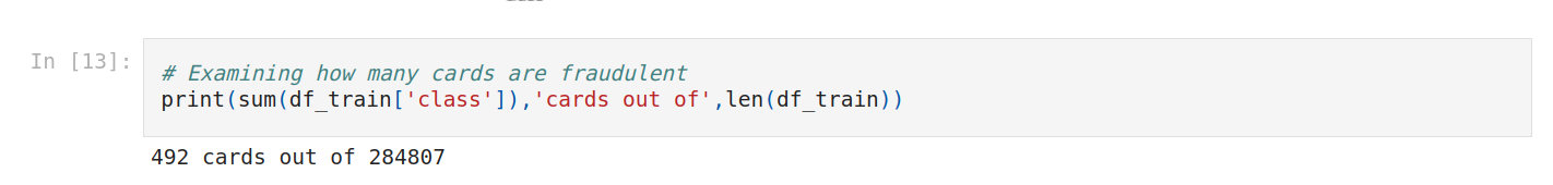
We can type how many cards are fraudulent.
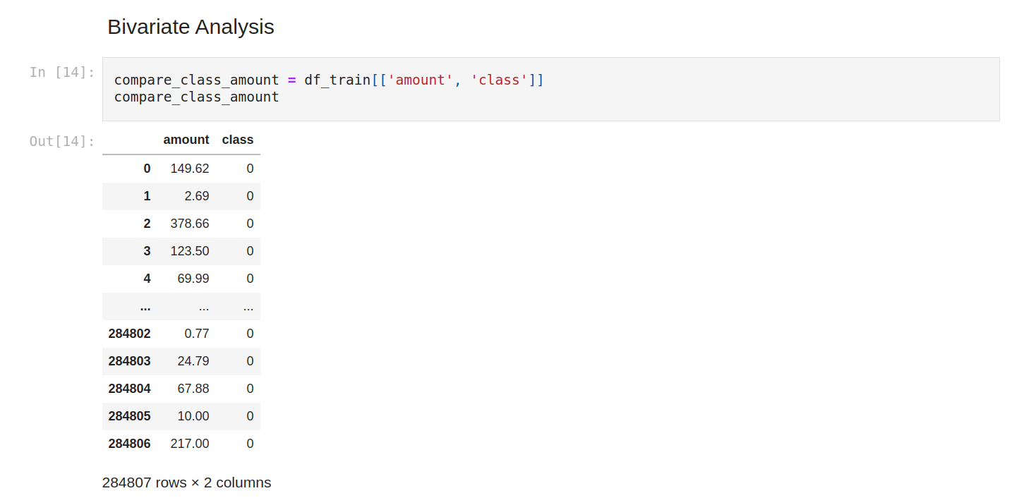
Bivariate Analysis requires you to learn about relationships between pairs of variables. We can use a scatter plot, a pair plot, or a correlation matrix.
We can for example compare amount with class.
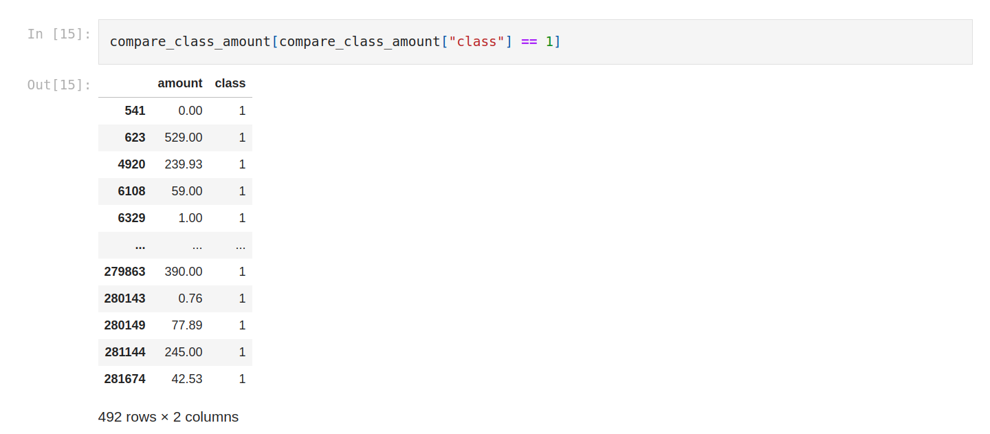
And filter to show only positive class. We can see that the amount is variable.
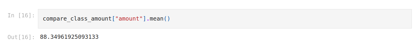
Let’s check the mean.
On average the fraud is 88.
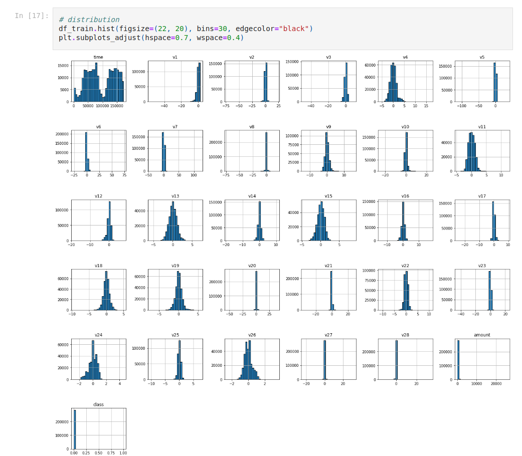
Let’s check the distribution with histograms.
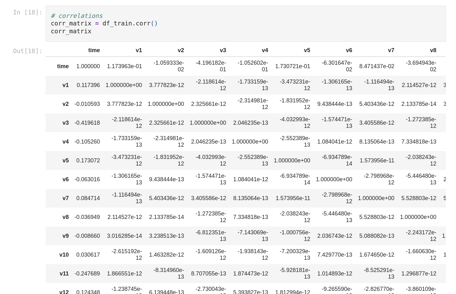
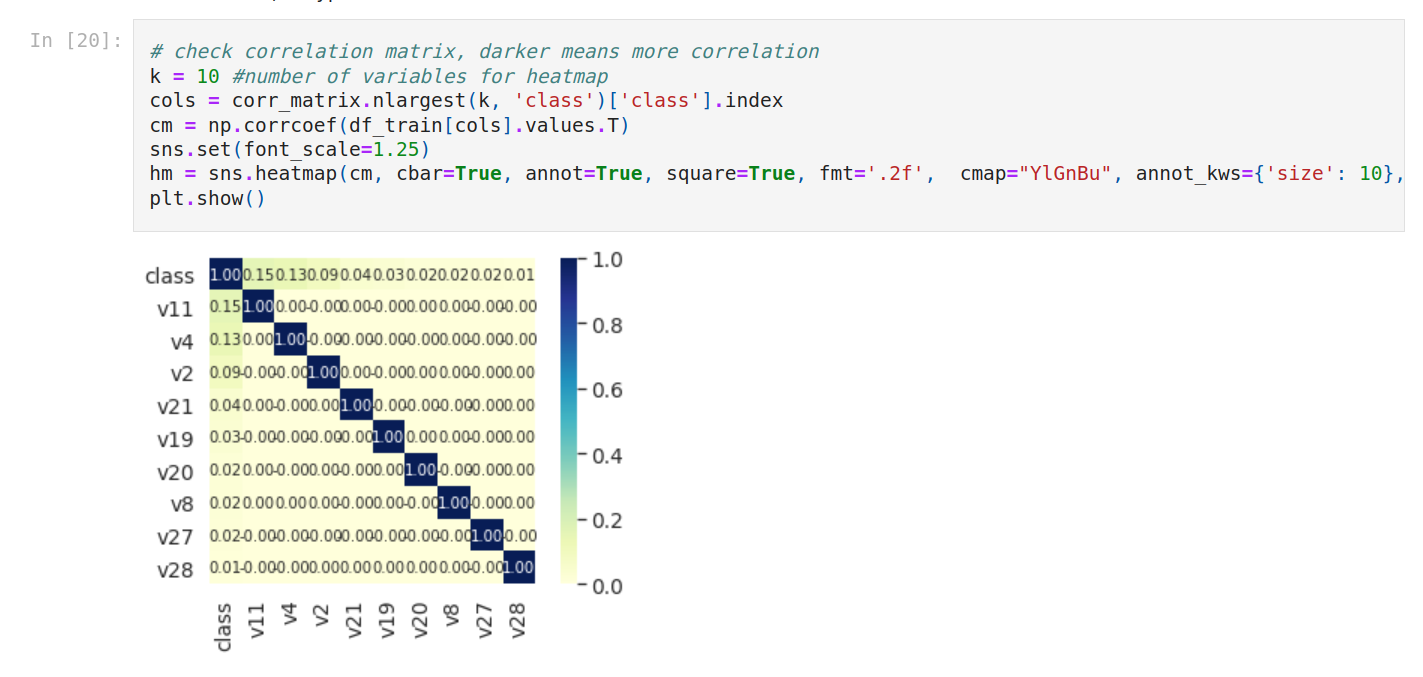
One thing we can do is to check correlations.
As usual; it’s better to plot it. We do that with a correlation matrix.
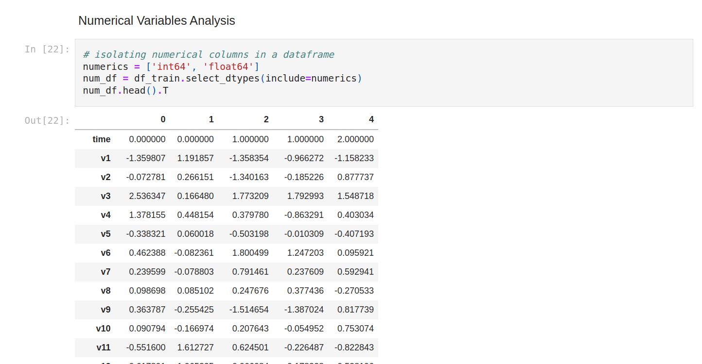
Now we’re gonna check outliers. We isolate numerical columns just to show you how to do that.
Let’s do again the summary statistics of all the columns.
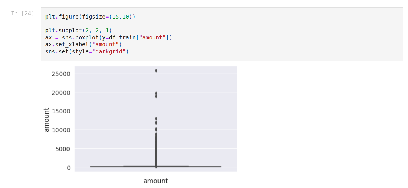
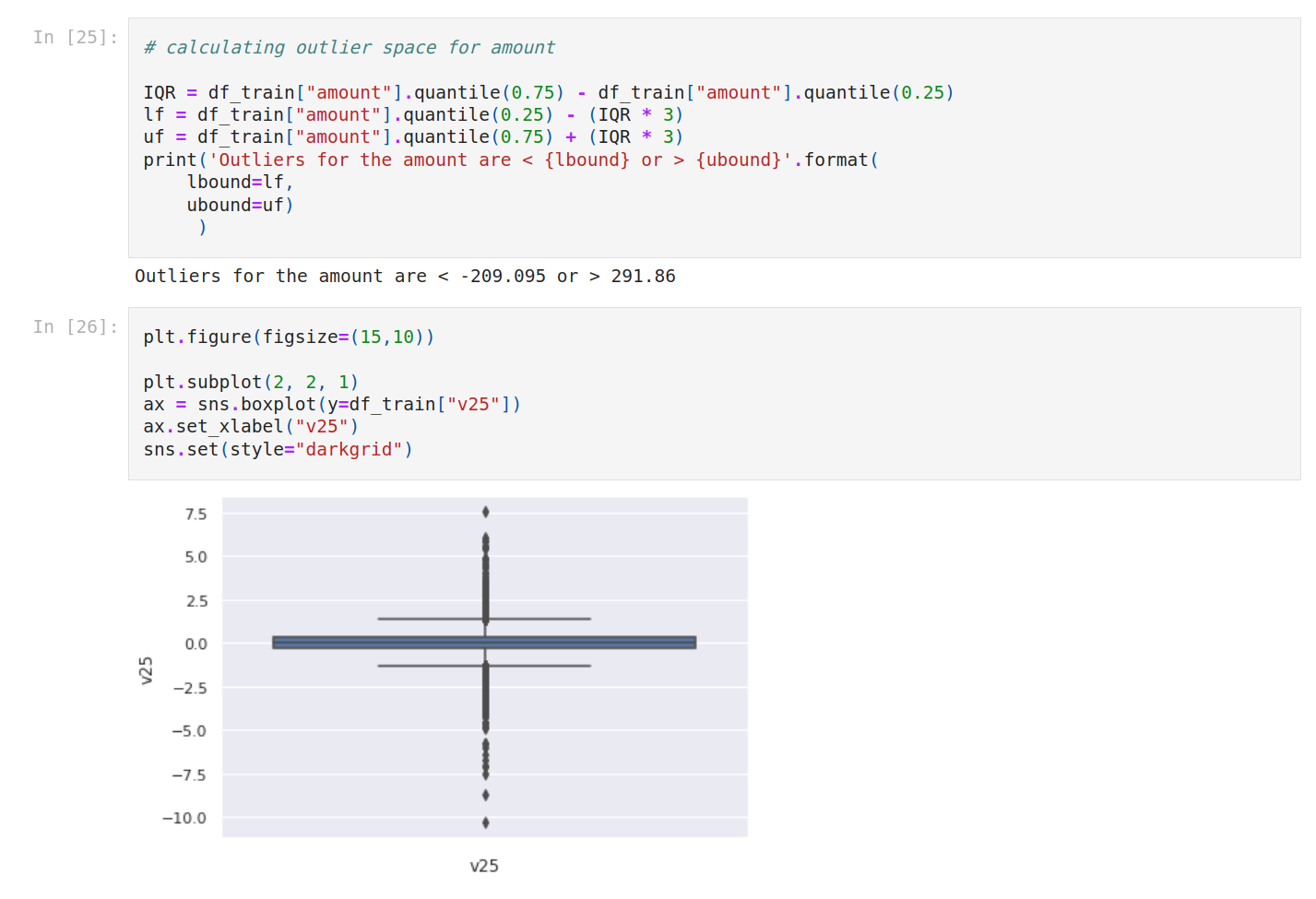
We can plot the outliers with boxplots. So we do that for amount and V25.
Also, we calculate outlier space for both.
Also, we calculate outlier space for both.
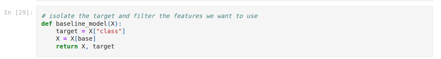
4. Baseline model
It’s time to create our baseline model. The goal is to have a quick idea about what we can get with just a few variables.
We select 5 variables and of course without the target.
So we create a function that we name baseline_model. The input is the dataset.
First we isolate the target from the target as usual (class). We get the features and we return the features and the target separately.
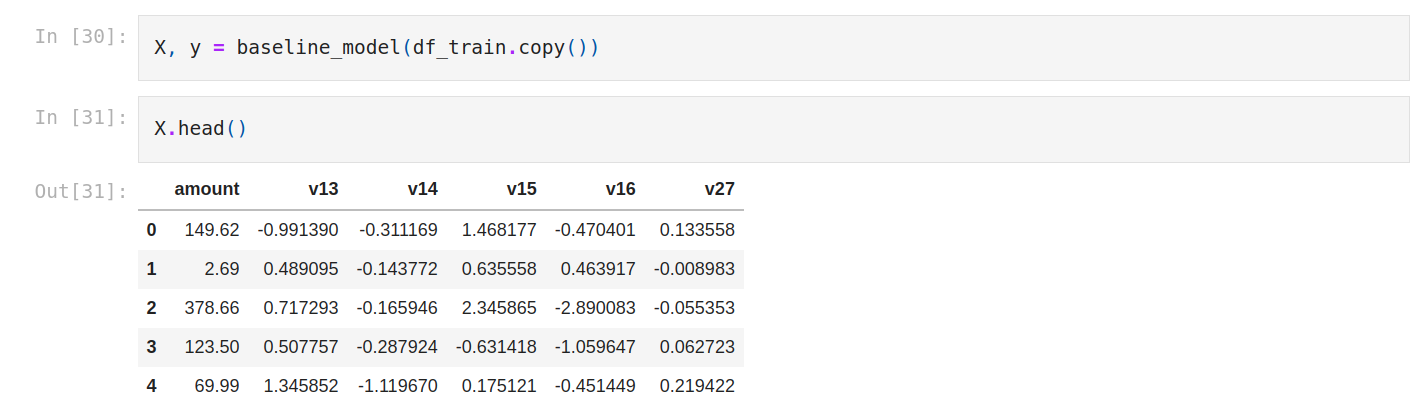
We create X and y.
Let’s check X.
Then, we import the logistic regression algorithm.
We instantiate the model, and we train it.
We make predictions.
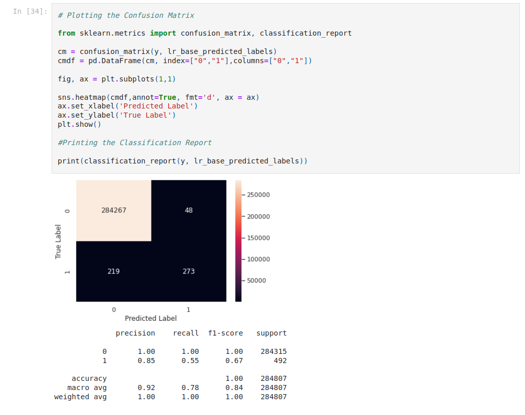
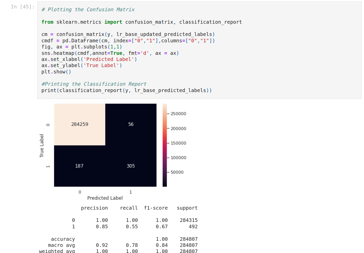
We’re gonna use the confusion matrix. A confusion matrix is a table that is used to define the performance of a classification algorithm.
Precision-Recall is a useful measure of the success of prediction when the classes are very imbalanced. In information retrieval, precision is a measure of result relevancy, while recall is a measure of how many truly relevant results are returned.
5. Feature engineering
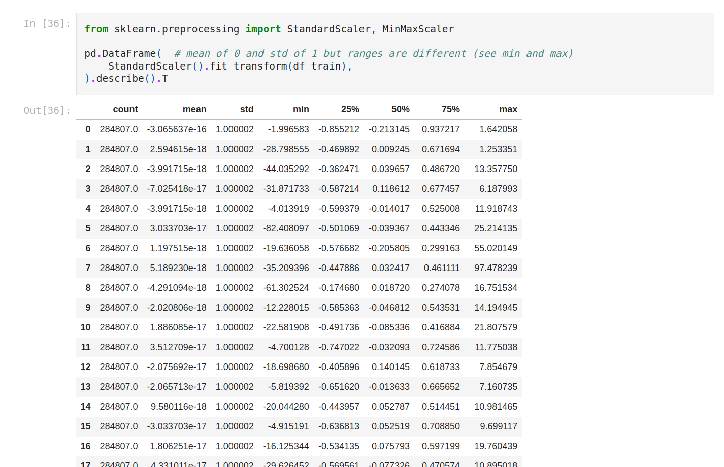
It’s time to do feature engineering. We start with feature scaling. let's use describe.
Mean, std, min and max are very different from each other, so let's standardize. We’re gonna use StandardScaler and MinMaxScaler.
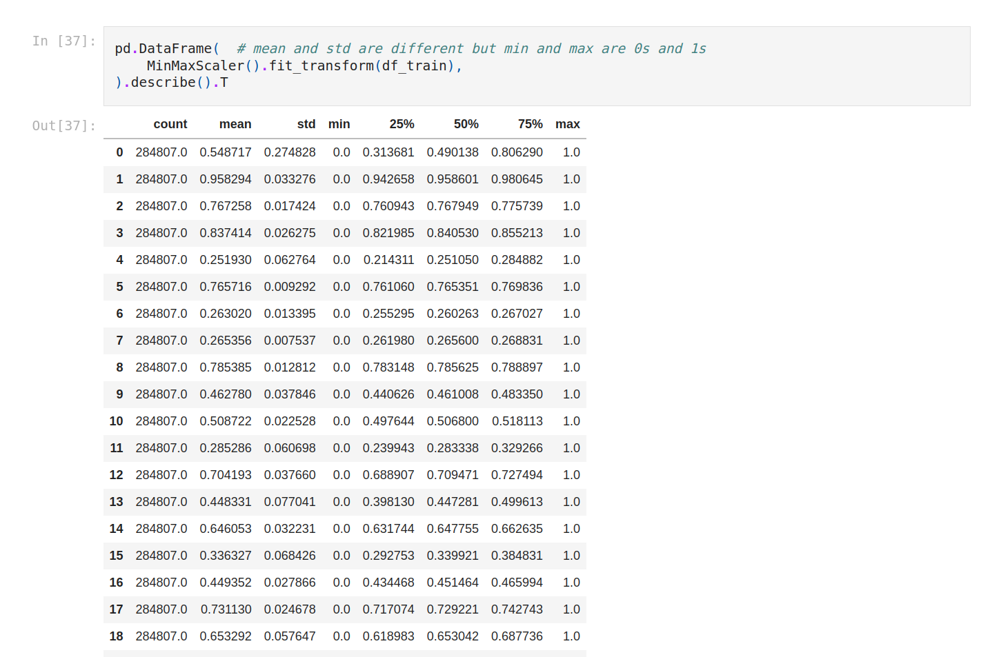
With MinMaxScaler everything is on the same scale.
Now we can update the model with the other features.
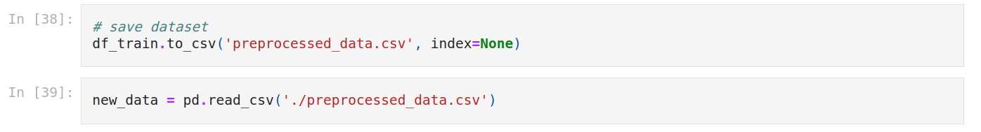
Let’s save the dataset. Now we get the new one.
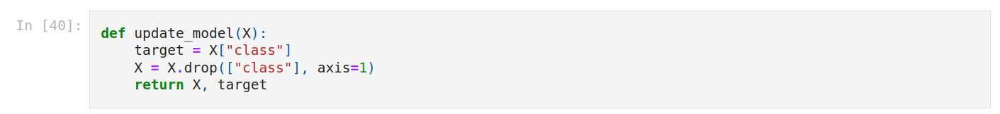
So we create a function named update_model. Pretty much the same as the first one but this time we drop class.
We update X and y.
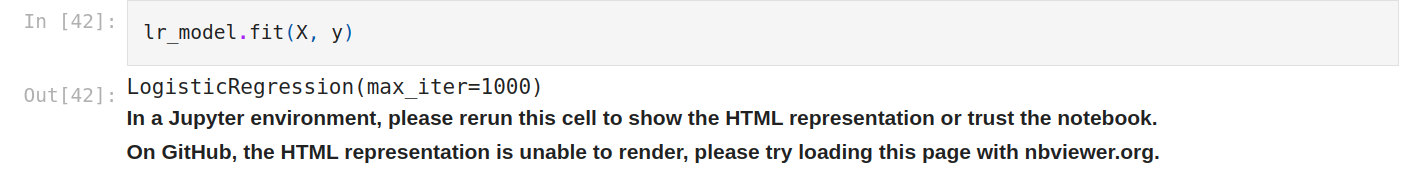
Then we fit the model.
We make predictions.
We plot again the confusion matrix. It seems worse.
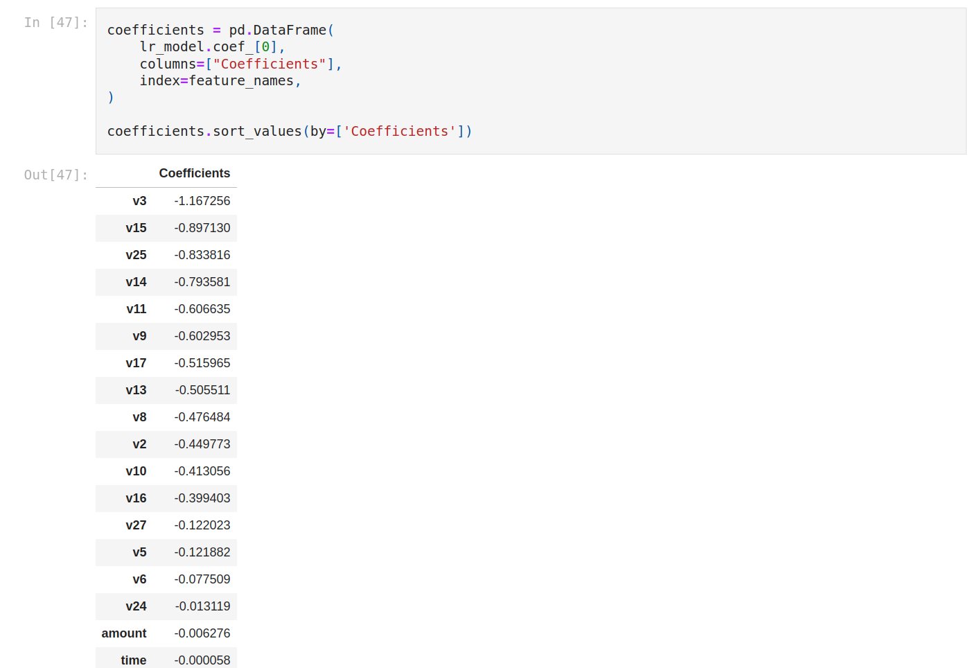
Let’s see the coefficients (weight of variables).
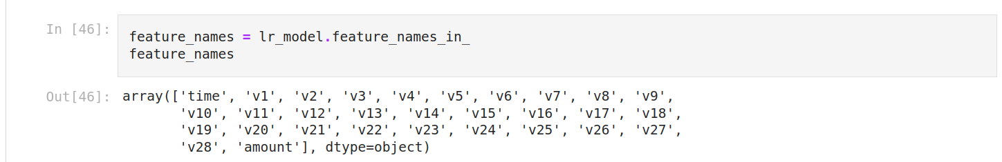
We’re gonna use feature_names_in_.
We can display an array and sort it.
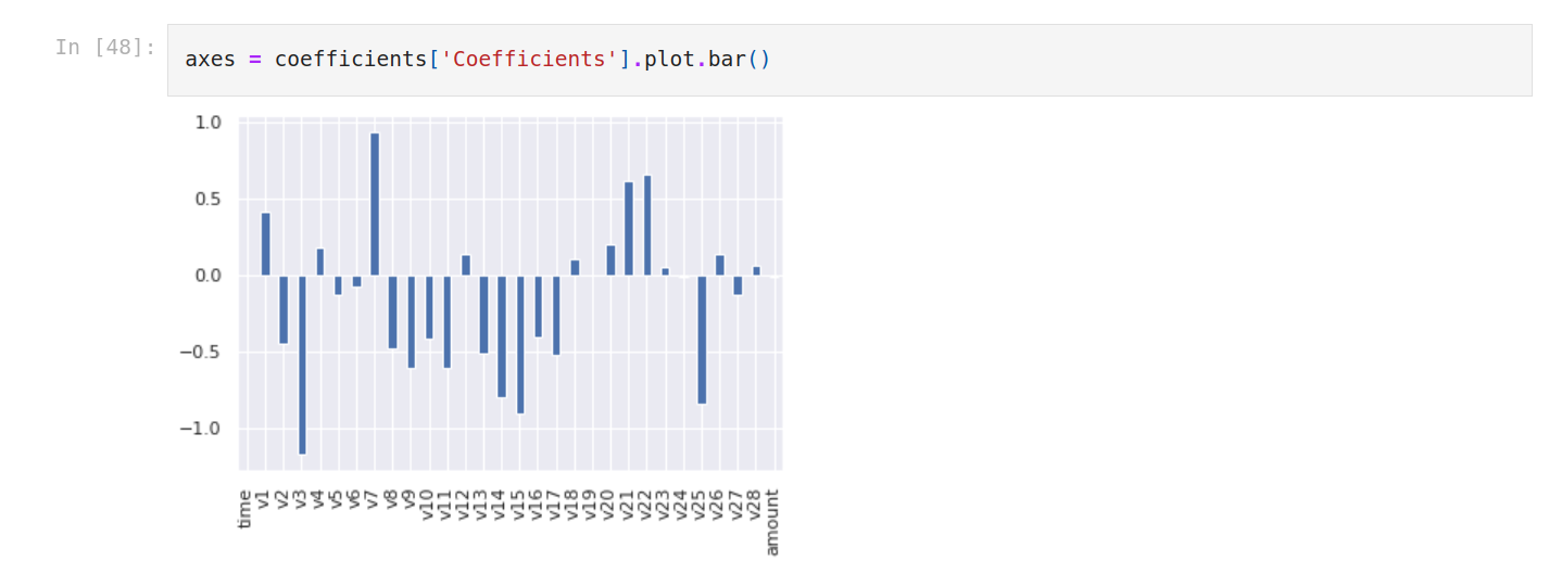
Let’s plot it to see better.
There are many very discriminating features especially V3, V15, V25 are very discriminating. amount is neutral. V7, V22 and V21 have a positive impact.
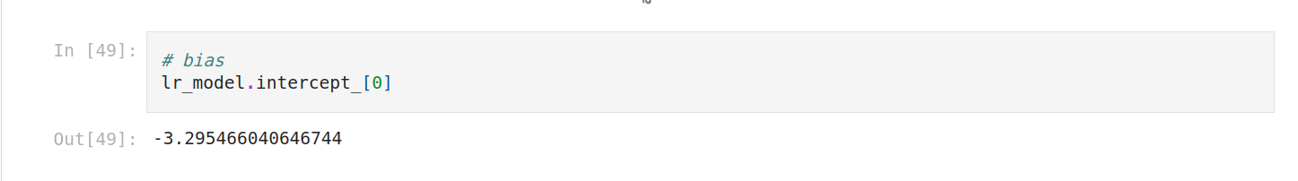
When we train our model on all features, the bias term is -3.29. The reason why the sign before the bias term is negative is the class balance. Meaning the probability of non-fraudulent on average is a little high.
This quiz aims to help you create a machine learning-powered chatbot tailored to your interests, passions, culture, values, and expertise area. Answer the following questions honestly to uncover your ideal chatbot concept.
Get tips to teach yourself data science without being overwelmed in your email box. Get secrets to think and act like a Data Scientist on a daily basis.
Don't leave without my signature FREE guide “Python for Data Science Quick Start" to learn the fundamentals of Python and how to use popular Data Science libraries.
Created with
Login or sign up to start learningLogin to start learning